Introduction
In modern society, medical image segmentation plays an essential role in developing
the medical system as it helps doctors to diagnose diseases and do surgical planning. There are many models developed for image segmentation, such as the U-net and the mask RCNN model. In this blog, we are going to introduce a novel model named TransUNet
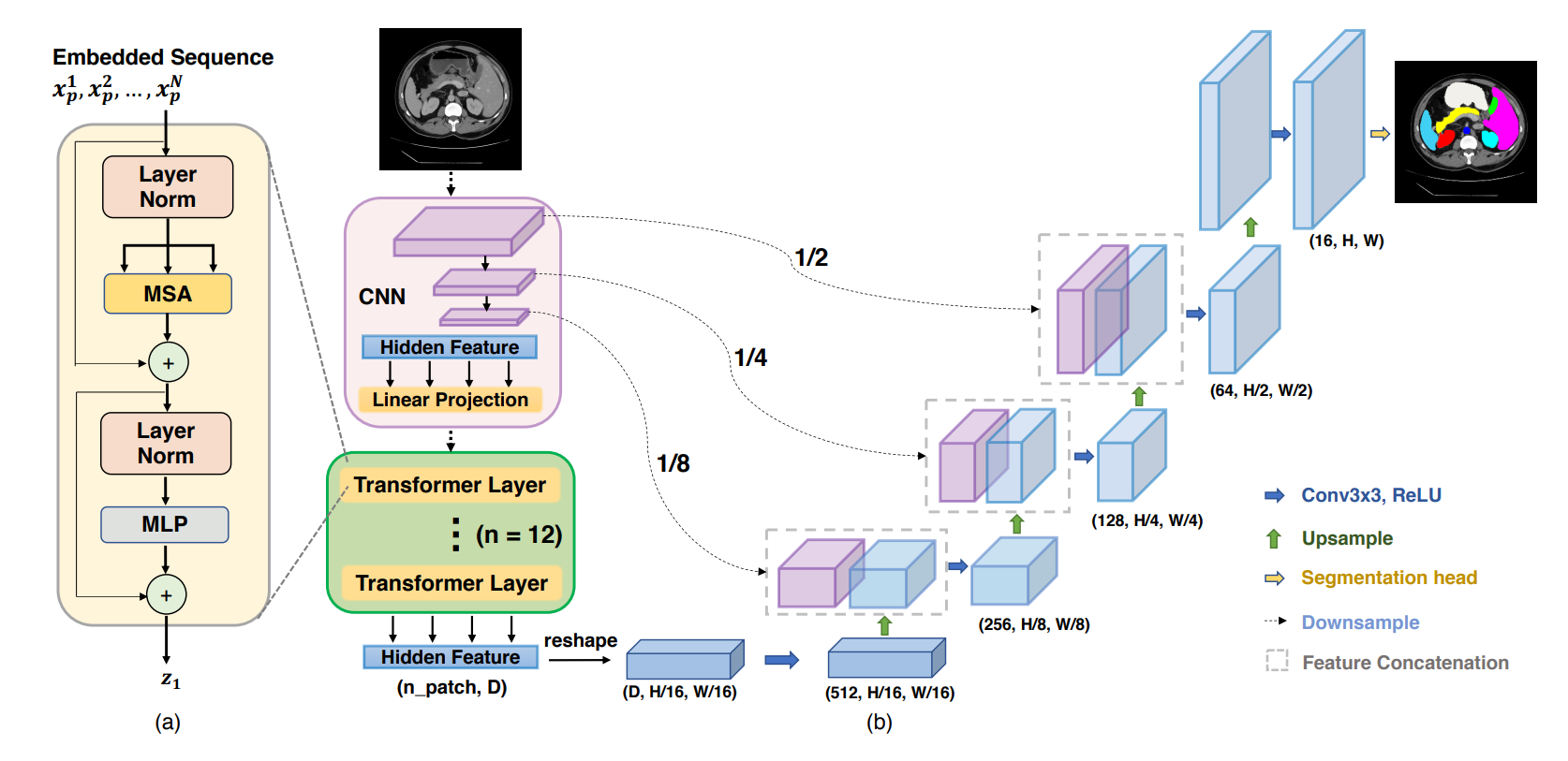
proposed by Chen et al. (2021) [1]. The figure above illustrates the structure of this model. Generally speaking, this model uses a CNN network (ResNet) and transformer blocks as the encoder and upsampling layers as the decoder to achieve the task. Although it looks quite complicated now, in this blog, we will divide the model into different parts and explain each part as detailed as possible.
Image segmentation denotes the process of partitioning images into several different segments. This is done per pixel. In other
words, we need to determine to which class each pixel belongs. The data needed for the image segmentation task should be
in the following form. For each image, there should be another image of the same size where each pixel represents to which class the corresponding pixel of the original image belongs. In other words, each data sample is a pair of image and its mask. The
mask is the ground truth label. In this paper, the authors used the Synapse multi-organ segmentation dataset. The images are
abdominal CT scans. The size of each slice of the CT scans is 512 times 512. There are eight different abdominal organ classes. Those are the aorta, gallbladder, left kidney, right kidney, liver, pancreas, spleen, and stomach. An additional class is used to represent pixels that belong to none of the organs mentioned above. Therefore, there are in total nine different classes. Now we are going to dive into the details of the model and explain them together with the codes.
Data loader
When using PyTorch to carry out a deep learning project, it is quite common to write a data loader for the model. The data
loader is used to load images, perform possible preprocessing or transformations on the images as approaches for data
augmentation. Two functions are defined to transform the images. The first function rotates the image 90 times k degrees, where k is a randomly generated integer between 0 and 3, including 3. It then flips the image given a random axis. The second function rotates the image given a random angle between (-20,20). It uses the spline interpolation to interpolate the pixels. Note that the same transformation done on an image should also be done on the corresponding mask image.
import os
import random
import h5py
import numpy as np
import torch
from PIL import Image
from scipy import ndimage
from scipy.ndimage.interpolation import zoom
from torch.utils.data import Dataset
def random_rot_flip(image, label):
    k = np.random.randint(0, 4)
    image = np.rot90(image, k)
    label = np.rot90(label, k)
    axis = np.random.randint(0, 2)
    image = np.flip(image, axis=axis).copy()
    label = np.flip(label, axis=axis).copy()
    return image, label


def random_rotate(image, label):
    angle = np.random.randint(-20, 20)
    image = ndimage.rotate(image, angle, order=0, reshape=False)
    label = ndimage.rotate(label, angle, order=0, reshape=False)
    return image, label
Researchers usually want to make some adjustments on input images by using torchvision.transforms. Transforms.Compose
is used to combine several actions. Here we could use some built-in functions of transform, like transforms.RandomCrop,
transforms.Normalize, or transforms.ToTensor. You could visit https://pytorch.org/vision/stable/transforms.html for more possible actions.
We could also personalize our own actions by implementing a __call__ function of a class. This will make our class
instance directly callable. As shown below, RandomGenerator is such a class. It first gets image and label,
which is actually two numpy ndarrays where the size equals to the original height and width of the data. Then it
performs rotation and flip on the images twice randomly. As what we have discussed above, it is used for the data augmentation.
After that, the array is zoomed using spline interpolation of the desired order. In other words, the size of the images
is changed. This is mainly because that the following network that we used, namely the ResNet, requires an input image
size of 224 times 224. Therefore, the original image size of 512 times 512 is not applicable anymore. For the mask images, since the pixel values (labels) are all integers and we need to keep this property after resizing, the order of 0
(the nearest interpolation) is used in the zoom() function. Finally, the modified images and mask images will be returned.
class RandomGenerator(object):
    def __init__(self, output_size):
        self.output_size = output_size

    def __call__(self, sample):
        image, label = sample['image'], sample['label']

        if random.random() > 0.5:
            image, label = random_rot_flip(image, label)
        elif random.random() > 0.5:
            image, label = random_rotate(image, label)
        x, y = image.shape
        if x != self.output_size[0] or y != self.output_size[1]:
            image = zoom(image, (self.output_size[0] / x, self.output_size[1] / y), order=3)
            label = zoom(label, (self.output_size[0] / x, self.output_size[1] / y), order=0)
        image = torch.from_numpy(image.astype(np.float32)).unsqueeze(0)
        label = torch.from_numpy(label.astype(np.float32))
        sample = {'image': image, 'label': label.long()}
        return sample
Now it's time to build our own data loader class. The class Synapse_dataset helps us load data from the dataset and apply possible preprocessing using the above functions. It inherits the Dataset class from torch.util.data, and we need to implement the __getitem__() function. In this function, we first need to find the file name of each data sample given the index and concatenate the data directory path with the file name. By doing such, we have got the path to access the data. Then we need to load data using np.load or h5py.File. The data sample is encapsulated in a dictionary data structure, in which the 'image' and 'label' are two keys. After acquiring the data, we could use the transform functions to do preprocessing. Similar to before, the modified images and masks are encapsulated in the dictionary data structure.
class Synapse_dataset(Dataset):
    def __init__(self, base_dir, list_dir, split, transform=None):
        self.transform = transform  # using transform in torch!
        self.split = split # test_data or train_data
        self.sample_list = open(os.path.join(list_dir, self.split+'.txt')).readlines()
        #we first get name of each data_sample
        self.data_dir = base_dir #dir of data

    def __len__(self):
        return len(self.sample_list)

    def __getitem__(self, idx):
        if self.split == "train":
            slice_name = self.sample_list[idx].strip('\n')
            data_path = os.path.join(self.data_dir, slice_name+'.npz')
            data = np.load(data_path)
            image, label = data['image'], data['label']
        else:
            vol_name = self.sample_list[idx].strip('\n')
            filepath = self.data_dir + "/{}.npy.h5".format(vol_name)
            data = h5py.File(filepath)
            image, label = data['image'][:], data['label'][:]

        sample = {'image': image, 'label': label}
        if self.transform:
            sample = self.transform(sample)
        sample['case_name'] = self.sample_list[idx].strip('\n')
        return sample
Now we have the data loader. It is time to use the data loader to read some images and masks and see what they look like, such that you will have a rough idea about the dataset. The following cell shows 64 images, in which there are 32 original medical images and 32 mask images. The odd columns represent the original images, and the even columns are the corresponding masks.
import matplotlib.pyplot as plt
import torchvision.utils as vutils

db_show = Synapse_dataset(base_dir='data/Synapse/train_npz', list_dir='./lists/lists_Synapse', split="train", transform=False)
showloader = DataLoader(db_show, batch_size=64, shuffle=True, num_workers=0, pin_memory=True)
real_batch = next(iter(showloader))
images = real_batch['image']
labels = real_batch['label']
data = []
for i in range(0, 32):
    data.append(images[i].unsqueeze(0))
    data.append(labels[i].unsqueeze(0))
plt.figure(figsize=(8, 8))
plt.axis("off")
plt.title("Training Images")
plt.imshow(np.transpose(vutils.make_grid(data, padding=2, normalize=True).cpu(), (1,2,0)))

Maybe the above images are not very clear. We will now show only one big image and its corresponding mask. The next cell does this job. The top image is the original CT scan, and the bottom one is the corresponding mask image. Different colors represent different organs in the mask image. Now I believe that you have got an idea about what the data look like. It's time to build the model and carry out the deep learning task.
def make_coloured(image):
    coloured_image = np.zeros((512, 512, 3))
    for i in range(0, 512):
        for j in range(0, 512):
            if image[i][j] == 0:
                coloured_image[i][j][0] = 0
                coloured_image[i][j][1] = 0
                coloured_image[i][j][2] = 0
            elif image[i][j] == 1:
                coloured_image[i][j][0] = 1
                coloured_image[i][j][1] = 0
                coloured_image[i][j][2] = 0
            elif image[i][j] == 2:
                coloured_image[i][j][0] = 0
                coloured_image[i][j][1] = 1
                coloured_image[i][j][2] = 0
            elif image[i][j] == 3:
                coloured_image[i][j][0] = 0
                coloured_image[i][j][1] = 0
                coloured_image[i][j][2] = 1
            elif image[i][j] == 4:
                coloured_image[i][j][0] = 1
                coloured_image[i][j][1] = 1
                coloured_image[i][j][2] = 0
            elif image[i][j] == 5:
                coloured_image[i][j][0] = 1
                coloured_image[i][j][1] = 0
                coloured_image[i][j][2] = 1
            elif image[i][j] == 6:
                coloured_image[i][j][0] = 0
                coloured_image[i][j][1] = 1
                coloured_image[i][j][2] = 1
            elif image[i][j] == 7:
                coloured_image[i][j][0] = 1
                coloured_image[i][j][1] = 0
                coloured_image[i][j][2] = 0.5
            elif image[i][j] == 8:
                coloured_image[i][j][0] = 0
                coloured_image[i][j][1] = 0.5
                coloured_image[i][j][2] = 1
    return coloured_image

data_path='case0005_slice063.npz'
data = np.load(data_path)
image_original=data['image'][:]
label_image=data['label'][:]
coloured_label =  make_coloured(label_image)

lb1 = Image.fromarray((coloured_label*255).astype(np.uint8))
im1 = Image.fromarray((image_original*255).astype(np.uint8))
lb_path='label1.bmp'
im_path='im1.bmp'
lb1.save(lb_path)
im1.save(im_path)

display(Image.open(im_path))
display(Image.open(lb_path))


Model architecture
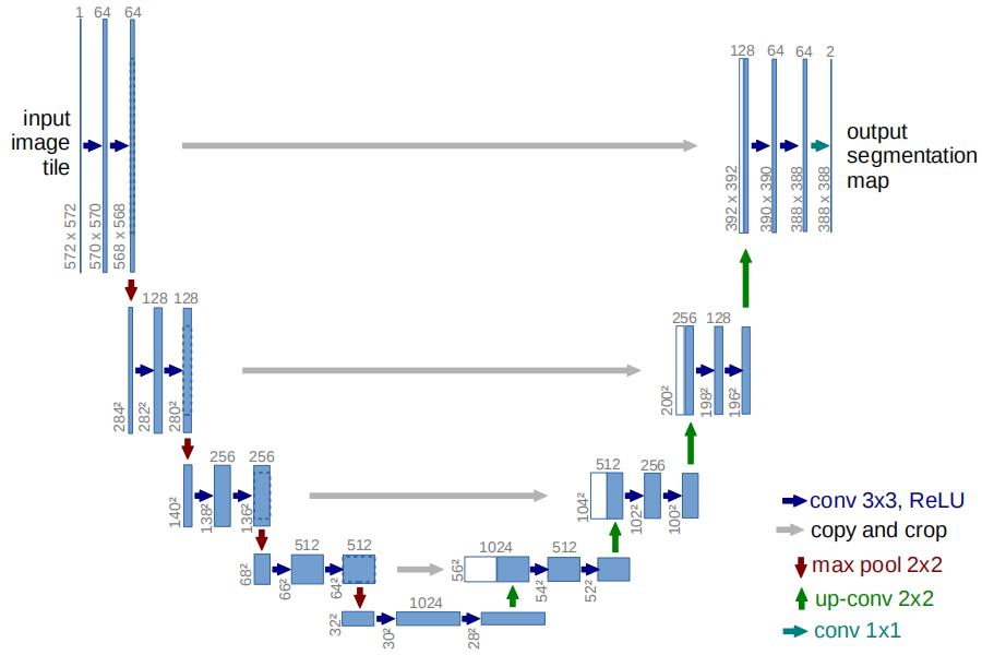
Now we are going to explain the overall model of Trans-UNet. It is inspired by the U-net [2] structure. U-net is a model that
was developed in 2015, aiming for biomedical image segmentation. It is a fully convolutional network (FCN). It can be divided
into two parts, the downsampling part and the upsampling part. In the downsampling part, several convolutional layers are used
to extract high-level features. However, unlike other one-direction convolutional neural networks, such as VGG-16 or AlexNet,
U-net stores the intermediate results after downsampling. When doing upsampling, the stored results are concatenated with the
upsampling results that have the same size. The image below clearly illustrates the structure of the U-net model. Being inspired by this model, Trans-UNet uses the residual network to extract features and do downsamplings. The results are then fed into a
transformer to encode. Afterwards, upsampling is used to decode the information.
ResNet
The residual network [3] is used to do downsamplings and extract high-level features in Trans-UNet. The advantage of ResNet
is that it can greatly alleviate the gradient vanishing problem by adding skip connections. In this project, the
ResNet-50 Vit-B_16 is used. The following function is used to load some useful parameters for the ResNet.
def get_r50_b16_config():
    """Returns the Resnet50 + ViT-B/16 configuration."""
    config = get_b16_config()
    config.patches.grid = (16, 16)
    config.resnet = ml_collections.ConfigDict()
    config.resnet.num_layers = (3, 4, 9)
    config.resnet.width_factor = 1

    config.classifier = 'seg'
    config.pretrained_path = '../model/vit_checkpoint/imagenet21k/R50+ViT-B_16.npz'
    config.decoder_channels = (256, 128, 64, 16)
    config.skip_channels = [512, 256, 64, 16]
    config.n_classes = 2
    config.n_skip = 3
    config.activation = 'softmax'

    return config
The following functions are used in ResNet. The np2th() function is used to transpose the images from the channel-last version to the channel-first version. The StdConv2d is a class that inherits the nn.Conv2d class. It extends the original 2d convolution operation by applying standard normalization on the weights. The function conv3x3() and conv1x1() are 2d convolutions with kernel size 3x3 and 1x1 using the StdConv2d operation.
from os.path import join as pjoin
from collections import OrderedDict

import torch
import torch.nn as nn
import torch.nn.functional as F

def np2th(weights, conv=False):
    """Possibly convert HWIO to OIHW."""
    if conv:
        weights = weights.transpose([3, 2, 0, 1])
    return torch.from_numpy(weights)

#standardize the weights before doing convolution
#weight -->(output_channel,input_channel,kernel_size[0],kernel_size[1])
#So compute mean and variance for each input_channel*kernel_size[0]*kernel_size[1]
class StdConv2d(nn.Conv2d):

    def forward(self, x):
        w = self.weight
        v, m = torch.var_mean(w, dim=[1, 2, 3], keepdim=True, unbiased=False)
        w = (w - m) / torch.sqrt(v + 1e-5)
        return F.conv2d(x, w, self.bias, self.stride, self.padding,
                        self.dilation, self.groups)

#do convolution using StdConv2d
def conv3x3(cin, cout, stride=1, groups=1, bias=False):
    return StdConv2d(cin, cout, kernel_size=3, stride=stride,
                     padding=1, bias=bias, groups=groups)


def conv1x1(cin, cout, stride=1, bias=False):
    return StdConv2d(cin, cout, kernel_size=1, stride=stride,
                     padding=0, bias=bias)
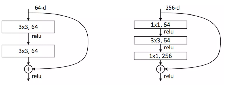
In this project, the bottleneck block is used in the ResNet. The following graph displays the normal ResNet block (on the left) and the bottleneck block (on the right). The key idea in bottleneck block is first using 1x1 kernels to decrease the number of channels, and then apply 3x3 kernels to do convolution as usual. In the end, it is necessary to apply 1x1 kernels again to get the channel number back to the origin. In the normal ResNet block, 1x1 convolution is not used. The bottleneck block allows the model to achieve the same thing as the normal block, with fewer parameters. Therefore, the bottleneck design is able to decrease the training time. It is worth mentioning another technique that is used here in this project, which is the group normalization. Before group normalization was proposed, researchers applied batch normalization between each hidden layer to alleviate the problems caused by internal covariate shift. However, when the batch size is small, batch normalization cannot perform very well. Group normalization divides the channels into groups and computes within each group the mean and variance for normalization. GN's computation is independent of the batch size, and its accuracy is stable in a wide range of batch sizes. Therefore, for small batch sizes, group normalization may outperform batch normalization. The cell below the figure denotes the bottleneck block. The load_from() function is used to load pre-trained weights for the model. It also appears in many other classes in this project.
class PreActBottleneck(nn.Module):
    """Pre-activation (v2) bottleneck block.
    """

    def __init__(self, cin, cout=None, cmid=None, stride=1):
        super().__init__()
        cout = cout or cin
        cmid = cmid or cout//4

        self.gn1 = nn.GroupNorm(32, cmid, eps=1e-6)
        self.conv1 = conv1x1(cin, cmid, bias=False)
        self.gn2 = nn.GroupNorm(32, cmid, eps=1e-6)
        self.conv2 = conv3x3(cmid, cmid, stride, bias=False)  # Original code has it on conv1!!
        self.gn3 = nn.GroupNorm(32, cout, eps=1e-6)
        self.conv3 = conv1x1(cmid, cout, bias=False)
        self.relu = nn.ReLU(inplace=True)

        if (stride != 1 or cin != cout):
            # Projection also with pre-activation according to paper.
            self.downsample = conv1x1(cin, cout, stride, bias=False)
            self.gn_proj = nn.GroupNorm(cout, cout)

    def forward(self, x):

        # Residual branch
        residual = x
        if hasattr(self, 'downsample'):
            residual = self.downsample(x)
            residual = self.gn_proj(residual)

        # Unit's branch
        y = self.relu(self.gn1(self.conv1(x)))
        y = self.relu(self.gn2(self.conv2(y)))
        y = self.gn3(self.conv3(y))

        y = self.relu(residual + y)
        return y

    def load_from(self, weights, n_block, n_unit):
        conv1_weight = np2th(weights[pjoin(n_block, n_unit, "conv1/kernel").replace('\\', '/')], conv=True)
        conv2_weight = np2th(weights[pjoin(n_block, n_unit, "conv2/kernel").replace('\\', '/')], conv=True)
        conv3_weight = np2th(weights[pjoin(n_block, n_unit, "conv3/kernel").replace('\\', '/')], conv=True)

        gn1_weight = np2th(weights[pjoin(n_block, n_unit, "gn1/scale").replace('\\', '/')])
        gn1_bias = np2th(weights[pjoin(n_block, n_unit, "gn1/bias").replace('\\', '/')])

        gn2_weight = np2th(weights[pjoin(n_block, n_unit, "gn2/scale").replace('\\', '/')])
        gn2_bias = np2th(weights[pjoin(n_block, n_unit, "gn2/bias").replace('\\', '/')])

        gn3_weight = np2th(weights[pjoin(n_block, n_unit, "gn3/scale").replace('\\', '/')])
        gn3_bias = np2th(weights[pjoin(n_block, n_unit, "gn3/bias").replace('\\', '/')])

        self.conv1.weight.copy_(conv1_weight)
        self.conv2.weight.copy_(conv2_weight)
        self.conv3.weight.copy_(conv3_weight)

        self.gn1.weight.copy_(gn1_weight.view(-1))
        self.gn1.bias.copy_(gn1_bias.view(-1))

        self.gn2.weight.copy_(gn2_weight.view(-1))
        self.gn2.bias.copy_(gn2_bias.view(-1))

        self.gn3.weight.copy_(gn3_weight.view(-1))
        self.gn3.bias.copy_(gn3_bias.view(-1))

        if hasattr(self, 'downsample'):
            proj_conv_weight = np2th(weights[pjoin(n_block, n_unit, "conv_proj/kernel").replace('\\', '/')], conv=True)
            proj_gn_weight = np2th(weights[pjoin(n_block, n_unit, "gn_proj/scale").replace('\\', '/')])
            proj_gn_bias = np2th(weights[pjoin(n_block, n_unit, "gn_proj/bias").replace('\\', '/')])

            self.downsample.weight.copy_(proj_conv_weight)
            self.gn_proj.weight.copy_(proj_gn_weight.view(-1))
            self.gn_proj.bias.copy_(proj_gn_bias.view(-1))
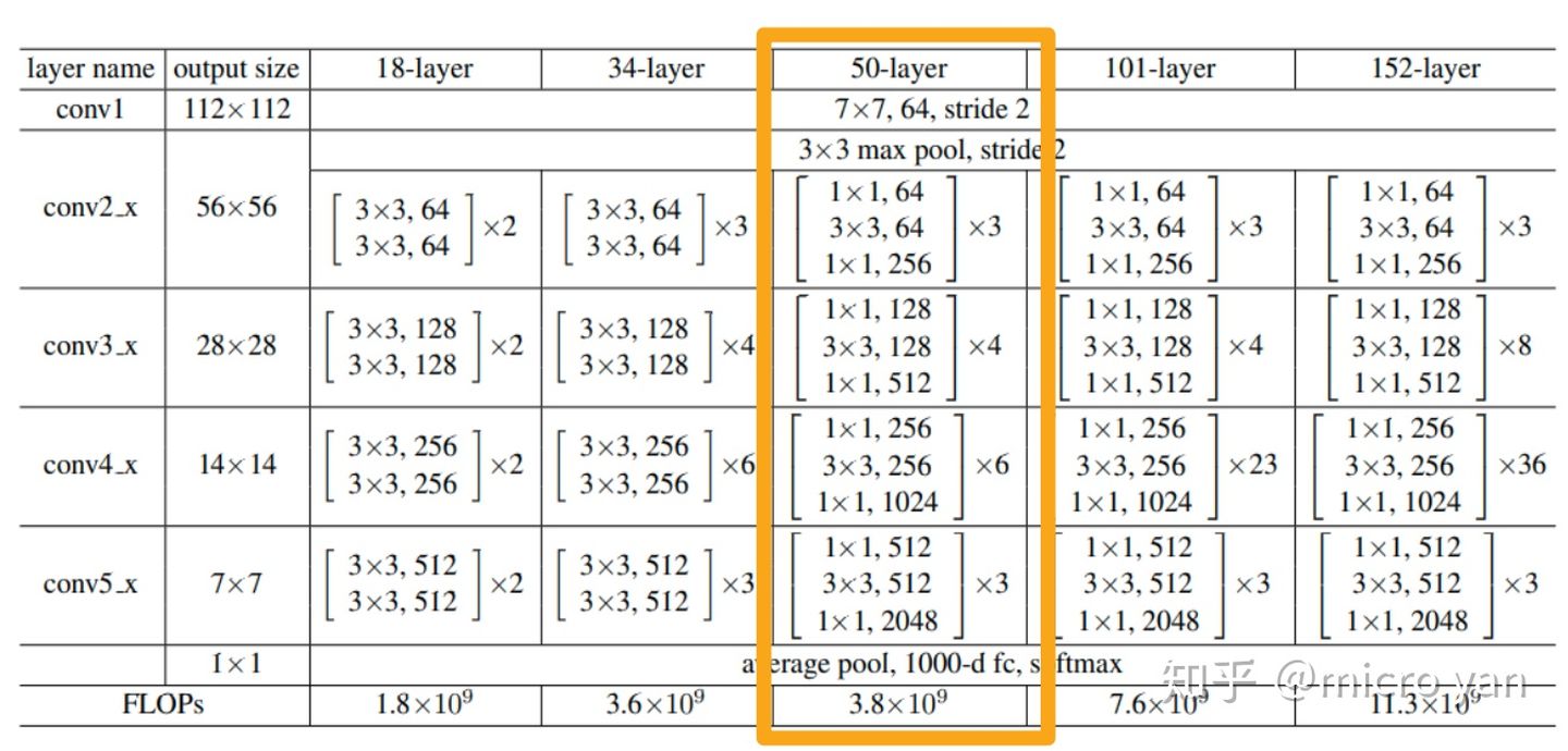
The Trans-UNet uses ResNet-50 as its backbone to get the feature map which is then used to form patches as the input of Vision Transformer. The structure of ResNet-50 that is used in this project is shown as the highlighted column in the figure below. The input images to the ResNet-50 are in the size of (3, 224, 224). This means that the height and width are 224 pixels, and there are three channels. The first convolutional layer use 64 7x7 kernels and a stride of 2, and the output images are in the size of (64, 112, 112). The images are then passed through a max-pooling layer, and the resulting images are in the size of (64, 56, 56). The rest of the ResNet-50 model consists of three successive bottleneck networks. The first part contains three bottleneck blocks, and the resulting images are in the size of (256, 56, 56). The second part consists of four bottleneck blocks, and the resulting images are in the size of (512, 28, 28). The last part consists of nine bottleneck blocks, and the resulting images are in the size of (1024, 14, 14). This last part is slightly different from what is shown in the figure below, but the overall structure is similar. In a nutshell, the input images to the ResNet-50 are 224x224 in 3 channels, while the output images are 14x14 in 1024 channels. The resulting images will then be used in the vision transformer model, where each pixel is an image patch, and there are in total 196 patches. The cell below implement the class ResNetV2. It is not hard to understand the structure now after the above explanation. The forward() function returns not only the resulting images but also a list named features, which stored all the intermediate results which will be used in the decoder (upsampling) part.
class ResNetV2(nn.Module):
    """Implementation of Pre-activation (v2) ResNet mode."""

    def __init__(self, block_units, width_factor):
        super().__init__()
        width = int(64 * width_factor)
        self.width = width

        self.root = nn.Sequential(OrderedDict([
            ('conv', StdConv2d(3, width, kernel_size=7, stride=2, bias=False, padding=3)),
            ('gn', nn.GroupNorm(32, width, eps=1e-6)),
            ('relu', nn.ReLU(inplace=True)),
            # ('pool', nn.MaxPool2d(kernel_size=3, stride=2, padding=0))
        ]))

        self.body = nn.Sequential(OrderedDict([
            ('block1', nn.Sequential(OrderedDict(
                [('unit1', PreActBottleneck(cin=width, cout=width*4, cmid=width))] +
                [(f'unit{i:d}', PreActBottleneck(cin=width*4, cout=width*4, cmid=width)) for i in range(2, block_units[0] + 1)],
                ))),
            ('block2', nn.Sequential(OrderedDict(
                [('unit1', PreActBottleneck(cin=width*4, cout=width*8, cmid=width*2, stride=2))] +
                [(f'unit{i:d}', PreActBottleneck(cin=width*8, cout=width*8, cmid=width*2)) for i in range(2, block_units[1] + 1)],
                ))),
            ('block3', nn.Sequential(OrderedDict(
                [('unit1', PreActBottleneck(cin=width*8, cout=width*16, cmid=width*4, stride=2))] +
                [(f'unit{i:d}', PreActBottleneck(cin=width*16, cout=width*16, cmid=width*4)) for i in range(2, block_units[2] + 1)],
                ))),
        ]))

    def forward(self, x):
        features = []
        b, c, in_size, _ = x.size()
        x = self.root(x)
        features.append(x)
        x = nn.MaxPool2d(kernel_size=3, stride=2, padding=0)(x)
        for i in range(len(self.body)-1):
            #According to paper, you have to concatenate the the output of resnet
            #blocks with decoder part so you have to make sure that the height and
            #width matches
            x = self.body[i](x)
            right_size = int(in_size / 4 / (i+1))
            if x.size()[2] != right_size:
                pad = right_size - x.size()[2]
                assert pad < 3 and pad > 0, "x {} should {}".format(x.size(), right_size)
                feat = torch.zeros((b, x.size()[1], right_size, right_size), device=x.device)
                feat[:, :, 0:x.size()[2], 0:x.size()[3]] = x[:]
            else:
                feat = x
            features.append(feat)
        x = self.body[-1](x)
        return x, features[::-1]
# coding=utf-8
from __future__ import absolute_import
from __future__ import division
from __future__ import print_function

import copy
import logging
import math
import ml_collections
from os.path import join as pjoin

import torch
import torch.nn as nn
import numpy as np

from torch.nn import CrossEntropyLoss, Dropout, Softmax, Linear, Conv2d, LayerNorm
from torch.nn.modules.utils import _pair
from scipy import ndimage
logger = logging.getLogger(__name__)
def get_b16_config():
    """Returns the ViT-B/16 configuration."""
    config = ml_collections.ConfigDict()
    config.patches = ml_collections.ConfigDict({'size': (16, 16)})
    config.hidden_size = 768
    config.transformer = ml_collections.ConfigDict()
    config.transformer.mlp_dim = 3072
    config.transformer.num_heads = 12
    config.transformer.num_layers = 12
    config.transformer.attention_dropout_rate = 0.0
    config.transformer.dropout_rate = 0.1

    config.classifier = 'seg'
    config.representation_size = None
    config.resnet_pretrained_path = None
    config.pretrained_path = '../model/vit_checkpoint/imagenet21k/ViT-B_16.npz'
    config.patch_size = 16

    config.decoder_channels = (256, 128, 64, 16)
    config.n_classes = 2
    config.activation = 'softmax'
    return config

def get_r50_b16_config():
    """Returns the Resnet50 + ViT-B/16 configuration."""
    config = get_b16_config()
    config.patches.grid = (16, 16)
    config.resnet = ml_collections.ConfigDict()
    config.resnet.num_layers = (3, 4, 9)
    config.resnet.width_factor = 1

    config.classifier = 'seg'
    config.pretrained_path = '../model/vit_checkpoint/imagenet21k/R50+ViT-B_16.npz'
    config.decoder_channels = (256, 128, 64, 16)
    config.skip_channels = [512, 256, 64, 16]
    config.n_classes = 2
    config.n_skip = 3
    config.activation = 'softmax'

    return config
CONFIGS = {
    'ViT-B_16': get_b16_config(),
    'R50-ViT-B_16': get_r50_b16_config(),

}
Vision Transformer
This part is about the transformer. We first need to get embeddings of the image patch to construct the inputs of the transformer model. Then, we build the attention block and the feed-forward network as the basic building block of the transformer model. We then stack these blocks to build the whole transformer model. The resulting transformer model, together with the ResNet model, forms the encoder of Trans-UNet.
Embedding layer
The resulting outputs of the previous ResNet-50 model are in the size of (1024, 14, 14). Each 'pixel' of the output can be seen as an image patch. Therefore, for each input image, after passing through the ResNet model, we could have 14x14=196 image patches. Each image patch has 1024 channels. We could also see each image patch as a vector with a length of 1024. In other words, we construct embeddings for each input image. The code in the following cell implements the embedding layer. The hybrid_model is the ResNet model. After getting the output from the ResNet model, there is a 2D convolution layer named patch_embeddings which decreases the number of channels from 1024 to 768. This is because that we need to apply self-attention later, and the input embeddings to the self-attention layer need to be in the length of 768. This is what the authors in the original self-attention paper did, and the same input size is applied here. Now each image's size is (768, 14, 14). We need to apply a flatten and a transpose operation on the image patches to make it become 2D. This is because that the original 3D data (768, 14, 14) cannot be used in the self-attention layer. Now, each input image has become a 2D matrix of size (196, 768). In other words, each image is represented by 196 vectors of size 768. These are the embeddings for each individual image. Drawing an analogy on the NLP task, we could think of a sentence that has 196 words, and each word is represented by an embedding vector of size 768. Now that we have the image embeddings, we could use the transformer model on it for encoding. Before feeding the embeddings into the transformer model, we need to add the position embeddings and apply the dropout technique.
class Embeddings(nn.Module):
    """Construct the embeddings from patch, position embeddings.
    """
    def __init__(self, config, img_size, in_channels=3):
        super(Embeddings, self).__init__()
        self.hybrid = None
        self.config = config
        img_size = _pair(img_size)
        #print(config.patches.get("grid"))
        #print(img_size)
        if config.patches.get("grid") is not None:   # ResNet
            grid_size = config.patches["grid"]
            #print(grid_size)
            patch_size = (img_size[0] // 16 // grid_size[0], img_size[1] // 16 // grid_size[1])
            patch_size_real = (patch_size[0] * 16, patch_size[1] * 16)
            #print(patch_size,patch_size_real)
            n_patches = (img_size[0] // patch_size_real[0]) * (img_size[1] // patch_size_real[1])

            self.hybrid = True
        else:
            patch_size = _pair(config.patches["size"])
            n_patches = (img_size[0] // patch_size[0]) * (img_size[1] // patch_size[1])
            self.hybrid = False

        if self.hybrid:
            self.hybrid_model = ResNetV2(block_units=config.resnet.num_layers, width_factor=config.resnet.width_factor)
            in_channels = self.hybrid_model.width * 16
        self.patch_embeddings = Conv2d(in_channels=in_channels,
                                       out_channels=config.hidden_size,
                                       kernel_size=patch_size,
                                       stride=patch_size)
        self.position_embeddings = nn.Parameter(torch.zeros(1, n_patches, config.hidden_size))

        self.dropout = Dropout(config.transformer["dropout_rate"])


    def forward(self, x):
        if self.hybrid:
            x, features = self.hybrid_model(x)
        else:
            features = None
        x = self.patch_embeddings(x)  # (B, hidden. n_patches^(1/2), n_patches^(1/2))
        x = x.flatten(2)
        x = x.transpose(-1, -2)  # (B, n_patches, hidden)

        embeddings = x + self.position_embeddings
        embeddings = self.dropout(embeddings)
        return embeddings, features
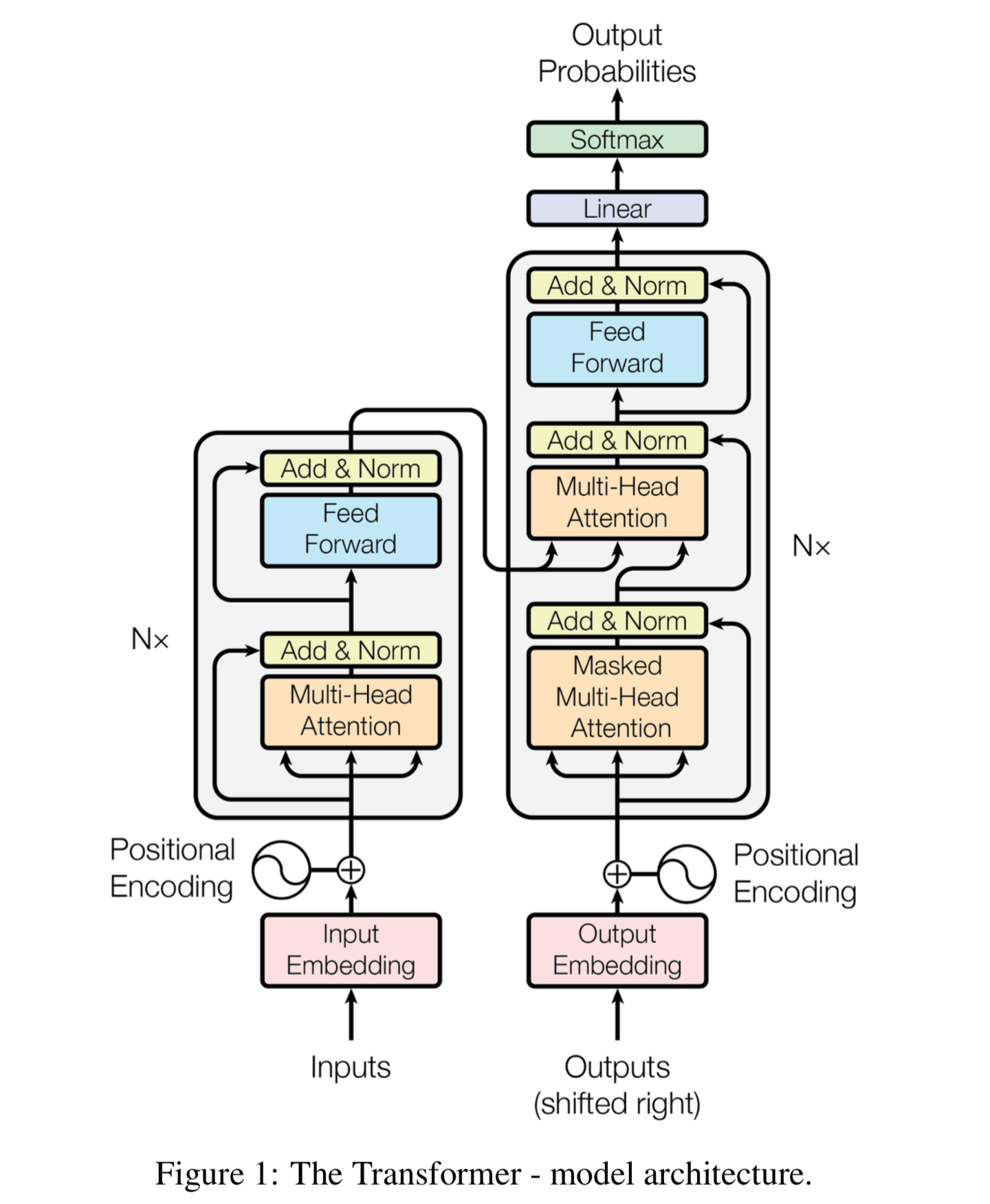
Transformer
The idea of the transformer model was first raised in 2014 on NLP tasks [4]. The model of transformer is illustrated in the figure below. In this project, we actually only apply the left part of the transformer model (the encoder part). It is a stacking of several transformer blocks. Each transformer block consists of a multi-head self-attention layer and a feedforward MLP layer. The self-attention layer helps the entire model to know where to focus. For each input x of size (196, 768), we apply matrix multiplication three times to get three matrices, the Q (query) matrix, K (key) matrix, and the V (value) matrix. The three matrices have the size of (196, 768). Since we are applying multi-head attention now, we need to divide the matrices into several different groups. The default setting is using 12 heads. Therefore, we now have 12 groups of Q, K, and V matrix, and the three matrices in each group have a size of (196, 64) (768/12=64). In each group, we need to use the following formula for
calculation.
$$
Attention(Q, K, V) = softmax(\frac{QK^T}{\sqrt(d_k)})V
$$
The matrix multiplication of Q and K calculates the similarity between each pair of the 196 embeddings. The result is then
divided by the squared root of the head size, which is 64 in this case. This division is used to mitigate the large-magnitude
problem caused by the large value of head size. Now we should have a matrix of size (196, 196). Each element represents the
similarity between two image patches. After applying the softmax function, we now could get the weights of all image patches
given each image patch. We then need to calculate the weighted sum over the values of all image patches for each image patch
to get the result. This is done by applying matrix multiplication again. After the above operations, the result is a matrix
of size (196, 64) for each head. Concatenating the results of all 12 heads and we get the final result of the multi-head
attention layer, which is a matrix of size (196, 768). Although the size remains the same, the information has been encoded.
Applying the idea from ResNet, the output is added with the input, and a layer normalization is applied. The result is then fed
into a multi-layer perceptron. It has only one hidden layer with 3072 neurons, and the output layer's size is 768. The idea of ResNet applies again, which is adding the input to the output and then apply the layer normalization. The
multi-head attention layer and the MLP layer together form the transformer's encoder block, and the result of each block is a matrix of size (196, 768). This matrix is then fed into the next block as the input. Twelve encoder blocks are used in total. The result of the final block is the encoded embeddings for an input image.
ATTENTION_Q = "MultiHeadDotProductAttention_1/query"
ATTENTION_K = "MultiHeadDotProductAttention_1/key"
ATTENTION_V = "MultiHeadDotProductAttention_1/value"
ATTENTION_OUT = "MultiHeadDotProductAttention_1/out"
FC_0 = "MlpBlock_3/Dense_0"
FC_1 = "MlpBlock_3/Dense_1"
ATTENTION_NORM = "LayerNorm_0"
MLP_NORM = "LayerNorm_2"


def np2th(weights, conv=False):
    """Possibly convert HWIO to OIHW."""
    if conv:
        weights = weights.transpose([3, 2, 0, 1])
    return torch.from_numpy(weights)


def swish(x):
    return x * torch.sigmoid(x)


ACT2FN = {"gelu": torch.nn.functional.gelu, "relu": torch.nn.functional.relu, "swish": swish}


class Attention(nn.Module):
    def __init__(self, config, vis):
        super(Attention, self).__init__()
        self.vis = vis
        self.num_attention_heads = config.transformer["num_heads"]
        self.attention_head_size = int(config.hidden_size / self.num_attention_heads)
        self.all_head_size = self.num_attention_heads * self.attention_head_size

        self.query = Linear(config.hidden_size, self.all_head_size)
        self.key = Linear(config.hidden_size, self.all_head_size)
        self.value = Linear(config.hidden_size, self.all_head_size)

        self.out = Linear(config.hidden_size, config.hidden_size)
        self.attn_dropout = Dropout(config.transformer["attention_dropout_rate"])
        self.proj_dropout = Dropout(config.transformer["attention_dropout_rate"])

        self.softmax = Softmax(dim=-1)

    def transpose_for_scores(self, x):
        new_x_shape = x.size()[:-1] + (self.num_attention_heads, self.attention_head_size)
        x = x.view(*new_x_shape)
        return x.permute(0, 2, 1, 3)

    def forward(self, hidden_states):
        mixed_query_layer = self.query(hidden_states)
        mixed_key_layer = self.key(hidden_states)
        mixed_value_layer = self.value(hidden_states)

        query_layer = self.transpose_for_scores(mixed_query_layer)
        key_layer = self.transpose_for_scores(mixed_key_layer)
        value_layer = self.transpose_for_scores(mixed_value_layer)

        attention_scores = torch.matmul(query_layer, key_layer.transpose(-1, -2))
        attention_scores = attention_scores / math.sqrt(self.attention_head_size)
        attention_probs = self.softmax(attention_scores)
        weights = attention_probs if self.vis else None
        attention_probs = self.attn_dropout(attention_probs)

        context_layer = torch.matmul(attention_probs, value_layer)
        context_layer = context_layer.permute(0, 2, 1, 3).contiguous()
        new_context_layer_shape = context_layer.size()[:-2] + (self.all_head_size,)
        context_layer = context_layer.view(*new_context_layer_shape)
        attention_output = self.out(context_layer)
        attention_output = self.proj_dropout(attention_output)
        return attention_output, weights
class Mlp(nn.Module):
    def __init__(self, config):
        super(Mlp, self).__init__()
        self.fc1 = Linear(config.hidden_size, config.transformer["mlp_dim"])
        self.fc2 = Linear(config.transformer["mlp_dim"], config.hidden_size)
        self.act_fn = ACT2FN["gelu"]
        self.dropout = Dropout(config.transformer["dropout_rate"])

        self._init_weights()

    def _init_weights(self):
        nn.init.xavier_uniform_(self.fc1.weight)
        nn.init.xavier_uniform_(self.fc2.weight)
        nn.init.normal_(self.fc1.bias, std=1e-6)
        nn.init.normal_(self.fc2.bias, std=1e-6)

    def forward(self, x):
        x = self.fc1(x)
        x = self.act_fn(x)
        x = self.dropout(x)
        x = self.fc2(x)
        x = self.dropout(x)
        return x
class Block(nn.Module):
    def __init__(self, config, vis):
        super(Block, self).__init__()
        self.hidden_size = config.hidden_size
        self.attention_norm = LayerNorm(config.hidden_size, eps=1e-6)
        self.ffn_norm = LayerNorm(config.hidden_size, eps=1e-6)
        self.ffn = Mlp(config)
        self.attn = Attention(config, vis)

    def forward(self, x):
        h = x
        x = self.attention_norm(x)
        x, weights = self.attn(x)
        x = x + h

        h = x
        x = self.ffn_norm(x)
        x = self.ffn(x)
        x = x + h
        return x, weights

    def load_from(self, weights, n_block):
        ROOT = f"Transformer/encoderblock_{n_block}"
        with torch.no_grad():
            Temp=weights
            query_weight = np2th(weights[pjoin(ROOT,ATTENTION_Q,"kernel").replace('\\', '/')]).view(self.hidden_size, self.hidden_size).t()

            key_weight = np2th(weights[pjoin(ROOT, ATTENTION_K, "kernel").replace('\\', '/')]).view(self.hidden_size, self.hidden_size).t()
            value_weight = np2th(weights[pjoin(ROOT, ATTENTION_V, "kernel").replace('\\', '/')]).view(self.hidden_size, self.hidden_size).t()
            out_weight = np2th(weights[pjoin(ROOT, ATTENTION_OUT, "kernel").replace('\\', '/')]).view(self.hidden_size, self.hidden_size).t()

            query_bias = np2th(weights[pjoin(ROOT, ATTENTION_Q, "bias").replace('\\', '/')]).view(-1)
            key_bias = np2th(weights[pjoin(ROOT, ATTENTION_K, "bias").replace('\\', '/')]).view(-1)
            value_bias = np2th(weights[pjoin(ROOT, ATTENTION_V, "bias").replace('\\', '/')]).view(-1)
            out_bias = np2th(weights[pjoin(ROOT, ATTENTION_OUT, "bias").replace('\\', '/')]).view(-1)

            self.attn.query.weight.copy_(query_weight)
            self.attn.key.weight.copy_(key_weight)
            self.attn.value.weight.copy_(value_weight)
            self.attn.out.weight.copy_(out_weight)
            self.attn.query.bias.copy_(query_bias)
            self.attn.key.bias.copy_(key_bias)
            self.attn.value.bias.copy_(value_bias)
            self.attn.out.bias.copy_(out_bias)

            mlp_weight_0 = np2th(weights[pjoin(ROOT, FC_0, "kernel").replace('\\', '/')]).t()
            mlp_weight_1 = np2th(weights[pjoin(ROOT, FC_1, "kernel").replace('\\', '/')]).t()
            mlp_bias_0 = np2th(weights[pjoin(ROOT, FC_0, "bias").replace('\\', '/')]).t()
            mlp_bias_1 = np2th(weights[pjoin(ROOT, FC_1, "bias").replace('\\', '/')]).t()

            self.ffn.fc1.weight.copy_(mlp_weight_0)
            self.ffn.fc2.weight.copy_(mlp_weight_1)
            self.ffn.fc1.bias.copy_(mlp_bias_0)
            self.ffn.fc2.bias.copy_(mlp_bias_1)

            self.attention_norm.weight.copy_(np2th(weights[pjoin(ROOT, ATTENTION_NORM, "scale").replace('\\', '/')]))
            self.attention_norm.bias.copy_(np2th(weights[pjoin(ROOT, ATTENTION_NORM, "bias").replace('\\', '/')]))
            self.ffn_norm.weight.copy_(np2th(weights[pjoin(ROOT, MLP_NORM, "scale").replace('\\', '/')]))
            self.ffn_norm.bias.copy_(np2th(weights[pjoin(ROOT, MLP_NORM, "bias").replace('\\', '/')]))
class Encoder(nn.Module):
    def __init__(self, config, vis):
        super(Encoder, self).__init__()
        self.vis = vis
        self.layer = nn.ModuleList()
        self.encoder_norm = LayerNorm(config.hidden_size, eps=1e-6)
        for _ in range(config.transformer["num_layers"]):
            layer = Block(config, vis)
            self.layer.append(copy.deepcopy(layer))

    def forward(self, hidden_states):


        attn_weights = []
        for layer_block in self.layer:
            hidden_states, weights = layer_block(hidden_states)
            if self.vis:
                attn_weights.append(weights)
        encoded = self.encoder_norm(hidden_states)
        return encoded, attn_weights
class Transformer(nn.Module):
    def __init__(self, config, img_size, vis):
        super(Transformer, self).__init__()
        self.embeddings = Embeddings(config, img_size=img_size)
        self.encoder = Encoder(config, vis)

    def forward(self, input_ids):
        embedding_output, features = self.embeddings(input_ids)
        encoded, attn_weights = self.encoder(embedding_output)  # (B, n_patch, hidden)
        return encoded, attn_weights, features
Decoder
Now we come to the decoder part. The decoder is relatively simple comparing with the encoder. The input to the decoder
is a matrix of size (196, 768). We first need to resize it to 3D to match the images. The size of the output after
resize is (768, 14, 14). Therefore we get the image representation back. We first need to apply a 2D convolution to change
the channel number. The result's size is (512, 14, 14). We do this because we need to concatenate the following results
with the stored intermediated results from the ResNet. It then passes through 4 decoder blocks. The decoder block first
performs upsampling with a factor of 2 and then concatenates the output with skip features from resnet50 middle layers. After passing through all the decoder blocks, the result's size is (16, 224, 224). We now need to apply the final convolution named
segmentation head to change the channel number equals to the number of classes, which is 9 in this case. Now we have got the
final output of the Trans-UNet model. The size is (9, 224, 224). Each pixel has nine channels, and each channel represents the
probability of that pixel belongs to a certain class after applying softmax.
class Conv2dReLU(nn.Sequential):
    def __init__(
            self,
            in_channels,
            out_channels,
            kernel_size,
            padding=0,
            stride=1,
            use_batchnorm=True,
    ):
        conv = nn.Conv2d(
            in_channels,
            out_channels,
            kernel_size,
            stride=stride,
            padding=padding,
            bias=not (use_batchnorm),
        )
        relu = nn.ReLU(inplace=True)

        bn = nn.BatchNorm2d(out_channels)

        super(Conv2dReLU, self).__init__(conv, bn, relu)
class DecoderBlock(nn.Module):
    def __init__(
            self,
            in_channels,
            out_channels,
            skip_channels=0,
            use_batchnorm=True,
    ):
        super().__init__()
        self.conv1 = Conv2dReLU(
            in_channels + skip_channels,
            out_channels,
            kernel_size=3,
            padding=1,
            use_batchnorm=use_batchnorm,
        )
        self.conv2 = Conv2dReLU(
            out_channels,
            out_channels,
            kernel_size=3,
            padding=1,
            use_batchnorm=use_batchnorm,
        )
        self.up = nn.UpsamplingBilinear2d(scale_factor=2)

    def forward(self, x, skip=None):
        x = self.up(x)
        if skip is not None:
            x = torch.cat([x, skip], dim=1)
        x = self.conv1(x)
        x = self.conv2(x)
        return x
class DecoderCup(nn.Module):
    def __init__(self, config):
        super().__init__()
        self.config = config
        head_channels = 512
        self.conv_more = Conv2dReLU(
            config.hidden_size,
            head_channels,
            kernel_size=3,
            padding=1,
            use_batchnorm=True,
        )
        decoder_channels = config.decoder_channels
        in_channels = [head_channels] + list(decoder_channels[:-1])
        out_channels = decoder_channels

        if self.config.n_skip != 0:
            skip_channels = self.config.skip_channels
            for i in range(4-self.config.n_skip):  # re-select the skip channels according to n_skip
                skip_channels[3-i]=0

        else:
            skip_channels=[0,0,0,0]

        blocks = [
            DecoderBlock(in_ch, out_ch, sk_ch) for in_ch, out_ch, sk_ch in zip(in_channels, out_channels, skip_channels)
        ]
        self.blocks = nn.ModuleList(blocks)

    def forward(self, hidden_states, features=None):
        B, n_patch, hidden = hidden_states.size()  # reshape from (B, n_patch, hidden) to (B, h, w, hidden)
        h, w = int(np.sqrt(n_patch)), int(np.sqrt(n_patch))
        x = hidden_states.permute(0, 2, 1)
        x = x.contiguous().view(B, hidden, h, w)
        x = self.conv_more(x)
        for i, decoder_block in enumerate(self.blocks):
            if features is not None:
                skip = features[i] if (i < self.config.n_skip) else None
            else:
                skip = None
            x = decoder_block(x, skip=skip)
        return x
class SegmentationHead(nn.Sequential):

    def __init__(self, in_channels, out_channels, kernel_size=3, upsampling=1):
        conv2d = nn.Conv2d(in_channels, out_channels, kernel_size=kernel_size, padding=kernel_size // 2)
        upsampling = nn.UpsamplingBilinear2d(scale_factor=upsampling) if upsampling > 1 else nn.Identity()
        super().__init__(conv2d, upsampling)
class VisionTransformer(nn.Module):
    def __init__(self, config, img_size=224, num_classes=21843, zero_head=False, vis=False):
        super(VisionTransformer, self).__init__()
        self.num_classes = num_classes
        self.zero_head = zero_head
        self.classifier = config.classifier
        self.transformer = Transformer(config, img_size, vis)
        self.decoder = DecoderCup(config)
        self.segmentation_head = SegmentationHead(
            in_channels=config['decoder_channels'][-1],
            out_channels=config['n_classes'],
            kernel_size=3,
        )
        self.config = config

    def forward(self, x):
        if x.size()[1] == 1:
            x = x.repeat(1,3,1,1)
        x, attn_weights, features = self.transformer(x)  # (B, n_patch, hidden)
        x = self.decoder(x, features)
        logits = self.segmentation_head(x)
        return logits

    def load_from(self, weights):
        with torch.no_grad():

            res_weight = weights
            self.transformer.embeddings.patch_embeddings.weight.copy_(np2th(weights["embedding/kernel"], conv=True))
            self.transformer.embeddings.patch_embeddings.bias.copy_(np2th(weights["embedding/bias"]))

            self.transformer.encoder.encoder_norm.weight.copy_(np2th(weights["Transformer/encoder_norm/scale"]))
            self.transformer.encoder.encoder_norm.bias.copy_(np2th(weights["Transformer/encoder_norm/bias"]))

            posemb = np2th(weights["Transformer/posembed_input/pos_embedding"])

            posemb_new = self.transformer.embeddings.position_embeddings
            if posemb.size() == posemb_new.size():
                self.transformer.embeddings.position_embeddings.copy_(posemb)
            elif posemb.size()[1]-1 == posemb_new.size()[1]:
                posemb = posemb[:, 1:]
                self.transformer.embeddings.position_embeddings.copy_(posemb)
            else:
                logger.info("load_pretrained: resized variant: %s to %s" % (posemb.size(), posemb_new.size()))
                ntok_new = posemb_new.size(1)
                if self.classifier == "seg":
                    _, posemb_grid = posemb[:, :1], posemb[0, 1:]
                gs_old = int(np.sqrt(len(posemb_grid)))
                gs_new = int(np.sqrt(ntok_new))
                print('load_pretrained: grid-size from %s to %s' % (gs_old, gs_new))
                posemb_grid = posemb_grid.reshape(gs_old, gs_old, -1)
                zoom = (gs_new / gs_old, gs_new / gs_old, 1)
                posemb_grid = ndimage.zoom(posemb_grid, zoom, order=1)  # th2np
                posemb_grid = posemb_grid.reshape(1, gs_new * gs_new, -1)
                posemb = posemb_grid
                self.transformer.embeddings.position_embeddings.copy_(np2th(posemb))

            # Encoder whole
            for bname, block in self.transformer.encoder.named_children():
                for uname, unit in block.named_children():
                    unit.load_from(weights, n_block=uname)

            if self.transformer.embeddings.hybrid:
                self.transformer.embeddings.hybrid_model.root.conv.weight.copy_(np2th(res_weight["conv_root/kernel"], conv=True))
                gn_weight = np2th(res_weight["gn_root/scale"]).view(-1)
                gn_bias = np2th(res_weight["gn_root/bias"]).view(-1)
                self.transformer.embeddings.hybrid_model.root.gn.weight.copy_(gn_weight)
                self.transformer.embeddings.hybrid_model.root.gn.bias.copy_(gn_bias)

                for bname, block in self.transformer.embeddings.hybrid_model.body.named_children():
                    for uname, unit in block.named_children():
                        unit.load_from(res_weight, n_block=bname, n_unit=uname)
Loss
Two losses are used in Trans-UNet. The first one is the cross-entropy loss, which is frequently used in classification tasks. The second loss is called the dice loss, which is commonly used in image segmentation tasks. Given the prediction X and
the ground truth label Y, the dice loss is calculated by the following formula. The multiplication here is element-wise, and the absolute value symbol here represents getting the sum of all elements in the matrix. The dice loss measures the similarity between the prediction and the ground truth mask. The total loss is the average value of the cross-entropy loss and the dice loss.
$$
DICE(X, Y) = 1 - \frac{2 * |X * Y| + smooth\ \ value}{|X*X| + |Y*Y| + smooth\ \ value}
$$
class DiceLoss(nn.Module):
    def __init__(self, n_classes):
        super(DiceLoss, self).__init__()
        self.n_classes = n_classes

    def _one_hot_encoder(self, input_tensor):
        tensor_list = []
        for i in range(self.n_classes):
            temp_prob = input_tensor == i  # * torch.ones_like(input_tensor)
            tensor_list.append(temp_prob.unsqueeze(1))
        output_tensor = torch.cat(tensor_list, dim=1)
        return output_tensor.float()

    def _dice_loss(self, score, target):
        target = target.float()
        smooth = 1e-5
        intersect = torch.sum(score * target)
        y_sum = torch.sum(target * target)
        z_sum = torch.sum(score * score)
        loss = (2 * intersect + smooth) / (z_sum + y_sum + smooth)
        loss = 1 - loss
        return loss

    def forward(self, inputs, target, weight=None, softmax=False):
        if softmax:
            inputs = torch.softmax(inputs, dim=1)
        target = self._one_hot_encoder(target)
        if weight is None:
            weight = [1] * self.n_classes
        assert inputs.size() == target.size(), 'predict {} & target {} shape do not match'.format(inputs.size(), target.size())
        class_wise_dice = []
        loss = 0.0
        for i in range(0, self.n_classes):
            dice = self._dice_loss(inputs[:, i], target[:, i])
            class_wise_dice.append(1.0 - dice.item())
            loss += dice * weight[i]
        return loss / self.n_classes
Training
Now we come to the training part of this project. We train the model for 150 epochs, and the batch size is set to 24. The
author of the original paper used stochastic gradient descent with momentum as the optimizer. After each training
iteration, the learning rate is decreased. After training, the model is saved, and we can then use the model for testing.
import argparse
import logging
import os
import random
import sys
import time
import numpy as np
import torch
import torch.nn as nn
import torch.optim as optim
from tensorboardX import SummaryWriter
from torch.nn.modules.loss import CrossEntropyLoss
from torch.utils.data import DataLoader
from tqdm import tqdm
from torchvision import transforms
def trainer_synapse(args, model, snapshot_path):
    logging.basicConfig(filename=snapshot_path + "/log.txt", level=logging.INFO,
                        format='[%(asctime)s.%(msecs)03d] %(message)s', datefmt='%H:%M:%S')
    logging.getLogger().addHandler(logging.StreamHandler(sys.stdout))
    logging.info(str(args))
    base_lr = args.base_lr
    num_classes = args.num_classes
    batch_size = args.batch_size * args.n_gpu
    # max_iterations = args.max_iterations
    db_train = Synapse_dataset(base_dir=args.root_path, list_dir=args.list_dir, split="train",
                               transform=transforms.Compose(
                                   [RandomGenerator(output_size=[args.img_size, args.img_size])]))
    print("The length of train set is: {}".format(len(db_train)))

    def worker_init_fn(worker_id):
        random.seed(args.seed + worker_id)

    trainloader = DataLoader(db_train, batch_size=batch_size, shuffle=True, num_workers=0, pin_memory=True,
                             worker_init_fn=worker_init_fn)
    if args.n_gpu > 1:
        model = nn.DataParallel(model)
    model.train()
    ce_loss = CrossEntropyLoss()
    dice_loss = DiceLoss(num_classes)
    optimizer = optim.SGD(model.parameters(), lr=base_lr, momentum=0.9, weight_decay=0.0001)
    writer = SummaryWriter(snapshot_path + '/log')
    iter_num = 0
    max_epoch = args.max_epochs
    max_iterations = args.max_epochs * len(trainloader)  # max_epoch = max_iterations // len(trainloader) + 1
    logging.info("{} iterations per epoch. {} max iterations ".format(len(trainloader), max_iterations))
    best_performance = 0.0
    iterator = tqdm(range(max_epoch), ncols=70)
    for epoch_num in iterator:
        for i_batch, sampled_batch in enumerate(trainloader):
            image_batch, label_batch = sampled_batch['image'], sampled_batch['label']
            image_batch, label_batch = image_batch.cuda(), label_batch.cuda()
            outputs = model(image_batch)
            loss_ce = ce_loss(outputs, label_batch[:].long())
            loss_dice = dice_loss(outputs, label_batch, softmax=True)
            loss = 0.5 * loss_ce + 0.5 * loss_dice
            optimizer.zero_grad()
            loss.backward()
            optimizer.step()
            lr_ = base_lr * (1.0 - iter_num / max_iterations) ** 0.9
            for param_group in optimizer.param_groups:
                param_group['lr'] = lr_

            iter_num = iter_num + 1
            writer.add_scalar('info/lr', lr_, iter_num)
            writer.add_scalar('info/total_loss', loss, iter_num)
            writer.add_scalar('info/loss_ce', loss_ce, iter_num)

            logging.info('iteration %d : loss : %f, loss_ce: %f' % (iter_num, loss.item(), loss_ce.item()))

            if iter_num % 20 == 0:
                image = image_batch[1, 0:1, :, :]
                image = (image - image.min()) / (image.max() - image.min())
                writer.add_image('train/Image', image, iter_num)
                outputs = torch.argmax(torch.softmax(outputs, dim=1), dim=1, keepdim=True)
                writer.add_image('train/Prediction', outputs[1, ...] * 50, iter_num)
                labs = label_batch[1, ...].unsqueeze(0) * 50
                writer.add_image('train/GroundTruth', labs, iter_num)

        save_interval = 50  # int(max_epoch/6)
        if epoch_num > int(max_epoch / 2) and (epoch_num + 1) % save_interval == 0:
            save_mode_path = os.path.join(snapshot_path, 'epoch_' + str(epoch_num) + '.pth')
            torch.save(model.state_dict(), save_mode_path)
            logging.info("save model to {}".format(save_mode_path))

        if epoch_num >= max_epoch - 1:
            save_mode_path = os.path.join(snapshot_path, 'epoch_' + str(epoch_num) + '.pth')
            torch.save(model.state_dict(), save_mode_path)
            logging.info("save model to {}".format(save_mode_path))
            iterator.close()
            break

    writer.close()
    return "Training Finished!"
import argparse
import logging
import os
import random
import numpy as np
import torch
import torch.backends.cudnn as cudnn
parser = argparse.ArgumentParser()
parser.add_argument('--root_path', type=str,
                    default='data/Synapse/train_npz', help='root dir for data')
parser.add_argument('--dataset', type=str,
                    default='Synapse', help='experiment_name')
parser.add_argument('--list_dir', type=str,
                    default='./lists/lists_Synapse', help='list dir')
parser.add_argument('--num_classes', type=int,
                    default=9, help='output channel of network')
parser.add_argument('--max_iterations', type=int,
                    default=30000, help='maximum epoch number to train')
parser.add_argument('--max_epochs', type=int,
                    default=150, help='maximum epoch number to train')
parser.add_argument('--batch_size', type=int,
                    default=24, help='batch_size per gpu')
parser.add_argument('--n_gpu', type=int, default=1, help='total gpu')
parser.add_argument('--deterministic', type=int,  default=1,
                    help='whether use deterministic training')
parser.add_argument('--base_lr', type=float,  default=0.01,
                    help='segmentation network learning rate')
parser.add_argument('--img_size', type=int,
                    default=224, help='input patch size of network input')
parser.add_argument('--seed', type=int,
                    default=1234, help='random seed')
parser.add_argument('--n_skip', type=int,
                    default=3, help='using number of skip-connect, default is num')
parser.add_argument('--vit_name', type=str,
                    default='R50-ViT-B_16', help='select one vit model')
parser.add_argument('--vit_patches_size', type=int,
                    default=16, help='vit_patches_size, default is 16')
args = parser.parse_args(args=['--root_path','data/Synapse/train_npz',
                               '--dataset','Synapse',
                               '--list_dir','./lists/lists_Synapse',
                               '--num_classes','9',
                               '--max_iterations','30000',
                               '--max_epochs','150',
                               '--batch_size','24',
                               '--n_gpu','1',
                               '--deterministic','1',
                               '--base_lr','0.01',
                               '--img_size','224',
                               '--seed','1234',
                               '--n_skip','3',
                               '--vit_name','R50-ViT-B_16',
                               '--vit_patches_size','16'])
print(args)
if not args.deterministic:
    cudnn.benchmark = True
    cudnn.deterministic = False
else:
    cudnn.benchmark = False
    cudnn.deterministic = True
print(args)
random.seed(args.seed)
np.random.seed(args.seed)
torch.manual_seed(args.seed)
torch.cuda.manual_seed(args.seed)
dataset_name = args.dataset
dataset_config = {
    'Synapse': {
        'root_path': 'data/Synapse/train_npz',
        'list_dir': 'lists/lists_Synapse',
        'num_classes': 9,
    },
}
if args.batch_size != 24 and args.batch_size % 6 == 0:
    args.base_lr *= args.batch_size / 24
args.num_classes = dataset_config[dataset_name]['num_classes']
args.root_path = dataset_config[dataset_name]['root_path']
args.list_dir = dataset_config[dataset_name]['list_dir']
args.is_pretrain = True
args.exp = 'TU_' + dataset_name + str(args.img_size)
snapshot_path = "model/{}/{}".format(args.exp, 'TU')
snapshot_path = snapshot_path + '_pretrain' if args.is_pretrain else snapshot_path
snapshot_path += '_' + args.vit_name
snapshot_path = snapshot_path + '_skip' + str(args.n_skip)
snapshot_path = snapshot_path + '_vitpatch' + str(args.vit_patches_size) if args.vit_patches_size!=16 else snapshot_path
snapshot_path = snapshot_path+'_'+str(args.max_iterations)[0:2]+'k' if args.max_iterations != 30000 else snapshot_path
snapshot_path = snapshot_path + '_epo' +str(args.max_epochs) if args.max_epochs != 30 else snapshot_path
snapshot_path = snapshot_path+'_bs'+str(args.batch_size)
snapshot_path = snapshot_path + '_lr' + str(args.base_lr) if args.base_lr != 0.01 else snapshot_path
snapshot_path = snapshot_path + '_'+str(args.img_size)
snapshot_path = snapshot_path + '_s'+str(args.seed) if args.seed!=1234 else snapshot_path
if not os.path.exists(snapshot_path):
    os.makedirs(snapshot_path)

config_vit = CONFIGS[args.vit_name]
#Use the configs.get_r50_b16_config()
#This step call get_b16_config() gives value to model parameters
#config = ml_collections.ConfigDict() to get parameters

config_vit.n_classes = args.num_classes
config_vit.n_skip = args.n_skip
#change the parameters for n_classes and n_skip
if args.vit_name.find('R50') != -1:
    config_vit.patches.grid = (int(args.img_size / args.vit_patches_size), int(args.img_size / args.vit_patches_size))
#in our first model R50+ViT-B_16.npz so the above if expression is true
#print(config_vit.pretrained_path)
net = VisionTransformer(config_vit, img_size=args.img_size, num_classes=config_vit.n_classes).cuda()

trainer = {'Synapse': trainer_synapse,}
trainer[dataset_name](args, net, snapshot_path)
Testing
Now we have already had the trained model, and we should use this model to make predictions on the testing dataset. The
performance is evaluated on two metrics, the average DSC and the Hausdorff distance (HD). A good model is supposed to have
a high average DSC value and a low HD value.
def calculate_metric_percase(pred, gt):
    pred[pred > 0] = 1
    gt[gt > 0] = 1
    if pred.sum() > 0 and gt.sum()>0:
        dice = metric.binary.dc(pred, gt)
        hd95 = metric.binary.hd95(pred, gt)
        return dice, hd95
    elif pred.sum() > 0 and gt.sum()==0:
        return 1, 0
    else:
        return 0, 0


def test_single_volume(image, label, net, classes, patch_size=[256, 256], test_save_path=None, case=None, z_spacing=1):
    image, label = image.squeeze(0).cpu().detach().numpy(), label.squeeze(0).cpu().detach().numpy()
    if len(image.shape) == 3:
        prediction = np.zeros_like(label)
        for ind in range(image.shape[0]):
            slice = image[ind, :, :]
            x, y = slice.shape[0], slice.shape[1]
            if x != patch_size[0] or y != patch_size[1]:
                slice = zoom(slice, (patch_size[0] / x, patch_size[1] / y), order=3)  # previous using 0
            input = torch.from_numpy(slice).unsqueeze(0).unsqueeze(0).float().cuda()
            net.eval()
            with torch.no_grad():
                outputs = net(input)
                out = torch.argmax(torch.softmax(outputs, dim=1), dim=1).squeeze(0)
                out = out.cpu().detach().numpy()
                if x != patch_size[0] or y != patch_size[1]:
                    pred = zoom(out, (x / patch_size[0], y / patch_size[1]), order=0)
                else:
                    pred = out
                prediction[ind] = pred
                if np.max(pred) != 0:
                    np.save('predictions/result_image_synapse/' + case + "_pred_", pred)
                    np.save('predictions/result_image_synapse/' + case + "_gt_", label)
    else:
        input = torch.from_numpy(image).unsqueeze(
            0).unsqueeze(0).float().cuda()
        net.eval()
        with torch.no_grad():
            out = torch.argmax(torch.softmax(net(input), dim=1), dim=1).squeeze(0)
            prediction = out.cpu().detach().numpy()
    metric_list = []
    for i in range(1, classes):
        metric_list.append(calculate_metric_percase(prediction == i, label == i))

    if test_save_path is not None:
        img_itk = sitk.GetImageFromArray(image.astype(np.float32))
        prd_itk = sitk.GetImageFromArray(prediction.astype(np.float32))
        lab_itk = sitk.GetImageFromArray(label.astype(np.float32))
        img_itk.SetSpacing((1, 1, z_spacing))
        prd_itk.SetSpacing((1, 1, z_spacing))
        lab_itk.SetSpacing((1, 1, z_spacing))
        sitk.WriteImage(prd_itk, test_save_path + '/'+case + "_pred.nii.gz")
        sitk.WriteImage(img_itk, test_save_path + '/'+ case + "_img.nii.gz")
        sitk.WriteImage(lab_itk, test_save_path + '/'+ case + "_gt.nii.gz")
    return metric_list
import argparse
import logging
import os
import random
import sys
import numpy as np
import torch
import torch.backends.cudnn as cudnn
import torch.nn as nn
from torch.utils.data import DataLoader
from tqdm import tqdm
from medpy import metric
from scipy.ndimage import zoom
import SimpleITK as sitk
parser = argparse.ArgumentParser()

parser.add_argument('--volume_path', type=str,
                    default='../data/Synapse/test_vol_h5', help='root dir for validation volume data')  # for acdc volume_path=root_dir
parser.add_argument('--dataset', type=str,
                    default='Synapse', help='experiment_name')
parser.add_argument('--num_classes', type=int,
                    default=4, help='output channel of network')
parser.add_argument('--list_dir', type=str,
                    default='./lists/lists_Synapse', help='list dir')

parser.add_argument('--max_iterations', type=int,default=20000, help='maximum epoch number to train')
parser.add_argument('--max_epochs', type=int, default=150, help='maximum epoch number to train')
parser.add_argument('--batch_size', type=int, default=24,
                    help='batch_size per gpu')
parser.add_argument('--img_size', type=int, default=224, help='input patch size of network input')
parser.add_argument('--is_savenii', action="store_true", help='whether to save results during inference', default=True)

parser.add_argument('--n_skip', type=int, default=3, help='using number of skip-connect, default is num')
parser.add_argument('--vit_name', type=str, default='R50-ViT-B_16', help='select one vit model')

parser.add_argument('--test_save_dir', type=str, default='predictions', help='saving prediction as nii!')
parser.add_argument('--deterministic', type=int,  default=1, help='whether use deterministic training')
parser.add_argument('--base_lr', type=float,  default=0.01, help='segmentation network learning rate')
parser.add_argument('--seed', type=int, default=1234, help='random seed')
parser.add_argument('--vit_patches_size', type=int, default=16, help='vit_patches_size, default is 16')

args = parser.parse_args(args=['--volume_path','data/Synapse/test_vol_h5',
                               '--dataset','Synapse',
                               '--num_classes','9',
                               '--list_dir','./lists/lists_Synapse',
                               '--max_iterations','20000',
                               '--max_epochs','150',
                               '--batch_size','24',
                               '--img_size','224',
                               '--n_skip', '3',
                               '--vit_name','R50-ViT-B_16',
                               '--test_save_dir', 'predictions',
                               '--deterministic', '1',
                               '--base_lr', '0.01',
                               '--seed','1234',
                               '--vit_patches_size','16',
                               ])
print(args)
def inference(args, model, test_save_path=None):
    db_test = args.Dataset(base_dir=args.volume_path, split="test_vol", list_dir=args.list_dir)
    testloader = DataLoader(db_test, batch_size=1, shuffle=False, num_workers=0)
    logging.info("{} test iterations per epoch".format(len(testloader)))
    model.eval()
    metric_list = 0.0
    for i_batch, sampled_batch in tqdm(enumerate(testloader)):
        h, w = sampled_batch["image"].size()[2:]
        image, label, case_name = sampled_batch["image"], sampled_batch["label"], sampled_batch['case_name'][0]
        metric_i = test_single_volume(image, label, model, classes=args.num_classes, patch_size=[args.img_size, args.img_size],
                                      test_save_path=test_save_path, case=case_name, z_spacing=args.z_spacing)
        metric_list += np.array(metric_i)
        logging.info('idx %d case %s mean_dice %f mean_hd95 %f' % (i_batch, case_name, np.mean(metric_i, axis=0)[0], np.mean(metric_i, axis=0)[1]))
    metric_list = metric_list / len(db_test)
    for i in range(1, args.num_classes):
        logging.info('Mean class %d mean_dice %f mean_hd95 %f' % (i, metric_list[i-1][0], metric_list[i-1][1]))
    performance = np.mean(metric_list, axis=0)[0]
    mean_hd95 = np.mean(metric_list, axis=0)[1]
    logging.info('Testing performance in best val model: mean_dice : %f mean_hd95 : %f' % (performance, mean_hd95))
    return "Testing Finished!"


if not args.deterministic:
    cudnn.benchmark = True
    cudnn.deterministic = False
else:
    cudnn.benchmark = False
    cudnn.deterministic = True
random.seed(args.seed)
np.random.seed(args.seed)
torch.manual_seed(args.seed)
torch.cuda.manual_seed(args.seed)

dataset_config = {
    'Synapse': {
        'Dataset': Synapse_dataset,
        'volume_path': 'data/Synapse/test_vol_h5',
        'list_dir': './lists/lists_Synapse',
        'num_classes': 9,
        'z_spacing': 1,
    },
}
dataset_name = args.dataset
args.num_classes = dataset_config[dataset_name]['num_classes']
args.volume_path = dataset_config[dataset_name]['volume_path']
args.Dataset = dataset_config[dataset_name]['Dataset']
args.list_dir = dataset_config[dataset_name]['list_dir']
args.z_spacing = dataset_config[dataset_name]['z_spacing']
args.is_pretrain = True

# name the same snapshot defined in train script!
args.exp = 'TU_' + dataset_name + str(args.img_size)
snapshot_path = "model/{}/{}".format(args.exp, 'TU')
snapshot_path = snapshot_path + '_pretrain' if args.is_pretrain else snapshot_path
snapshot_path += '_' + args.vit_name
snapshot_path = snapshot_path + '_skip' + str(args.n_skip)
snapshot_path = snapshot_path + '_vitpatch' + str(args.vit_patches_size) if args.vit_patches_size!=16 else snapshot_path
snapshot_path = snapshot_path + '_epo' + str(args.max_epochs) if args.max_epochs != 30 else snapshot_path
if dataset_name == 'ACDC':  # using max_epoch instead of iteration to control training duration
    snapshot_path = snapshot_path + '_' + str(args.max_iterations)[0:2] + 'k' if args.max_iterations != 30000 else snapshot_path
snapshot_path = snapshot_path+'_bs'+str(args.batch_size)
snapshot_path = snapshot_path + '_lr' + str(args.base_lr) if args.base_lr != 0.01 else snapshot_path
snapshot_path = snapshot_path + '_'+str(args.img_size)
snapshot_path = snapshot_path + '_s'+str(args.seed) if args.seed!=1234 else snapshot_path

config_vit = CONFIGS[args.vit_name]
config_vit.n_classes = args.num_classes
config_vit.n_skip = args.n_skip
config_vit.patches.size = (args.vit_patches_size, args.vit_patches_size)
if args.vit_name.find('R50') !=-1:
    config_vit.patches.grid = (int(args.img_size/args.vit_patches_size), int(args.img_size/args.vit_patches_size))
net = VisionTransformer(config_vit, img_size=args.img_size, num_classes=config_vit.n_classes).cuda()

snapshot = os.path.join(snapshot_path, 'best_model.pth')
if not os.path.exists(snapshot): snapshot = snapshot.replace('best_model', 'epoch_'+str(args.max_epochs-1))
net.load_state_dict(torch.load(snapshot.replace('\\', '/')))
snapshot_name = snapshot_path.split('/')[-1]

log_folder = './test_log/test_log_' + args.exp
os.makedirs(log_folder, exist_ok=True)
logging.basicConfig(filename=log_folder + '/'+snapshot_name+".txt", level=logging.INFO, format='[%(asctime)s.%(msecs)03d] %(message)s', datefmt='%H:%M:%S')
logging.getLogger().addHandler(logging.StreamHandler(sys.stdout))
logging.info(str(args))
logging.info(snapshot_name)

if args.is_savenii:
    args.test_save_dir = 'predictions'
    test_save_path = os.path.join(args.test_save_dir, args.exp, snapshot_name)
    os.makedirs(test_save_path, exist_ok=True)
else:
    test_save_path = None
inference(args, net, test_save_path)
Result
Now we have finished the testing. We tested the model on 12 CT scans. The first row of the table below shows the average DSC
value and the HD value of the testing results. It also displays the average DSC value on the eight different organs.
The second row shows the performance of the Trans-UNet in the original paper. We could see that there are only slight
differences between the two results. In conclusion, we have reproduced the model successfully.
| DSC | HD | Aorta | Gallbladder | Kidney (L) | Kidney (R) | Liver | Pancreas | Spleen | Stomach | |
|---|---|---|---|---|---|---|---|---|---|---|
| Our result | 76.92 | 33.38 | 86.67 | 57.15 | 82.04 | 78.21 | 94.89 | 54.89 | 85.12 | 76.41 |
| Original result | 77.48 | 31.69 | 87.23 | 63.13 | 81.87 | 77.02 | 94.08 | 55.86 | 85.08 | 75.62 |
Now let me show you directly the comparison between our predictions and the ground truth label. Again, we select one CT scan slice. The top image is the ground truth label, while the bottom image is the prediction that the model gives. Although there are slight differences, the model returns an acceptable result. Note that the edges of the organs in the prediction image are not as smooth as the ground truth image. This is because that we resize the prediction image from (224, 224) back to (512, 512).
gt = np.load('predictions/result_image/case0029_gt_60.npy')
gt = make_coloured(gt)
gt = Image.fromarray(np.uint8(gt*255))
gt_path='gt1.bmp'
gt.save(gt_path)
display(Image.open(gt_path))

pred = np.load('predictions/result_image/case0029_pred_60.npy')
pred = make_coloured(pred)
pred = Image.fromarray(np.uint8(pred*255))
pred_path='pred1.bmp'
pred.save(pred_path)
display(Image.open(pred_path))


Extension: Different optimizers
From this section, we will introduce some extensions that we did in addition to the original paper. We noticed that the authors of the original paper used stochastic gradient descent with momentum as the optimizer. We wonder that will the performance be improved if we use different optimizers. Therefore, the first extension that we did is trying different optimizers. We tried three other optimizers in total, namely RMSprop, Adadelta, and Adam. The following image shows the learning curve (the loss as a function of epoch number) of the three new optimizers and the original SGD optimizer. We can see that the SGD optimizer converges faster than the other optimizers, and its final loss is the lowest.
import matplotlib.pyplot as plt

def get_loss(file_path):
    with open(file_path, 'r') as f:
        content = f.readlines()
        total = 0
        loss = [0] * 150
        for i in range(0, 13950):
            total += float(content[i].split(' ')[6][:-1])
            if (i+1) % 93 == 0:
                loss[i // 93] = total / 93
                total = 0
    return loss

x = list(range(1, 151))
sgd_loss = get_loss('sgd_log.txt')
rmsprop_loss = get_loss('rmsprop_log.txt')
adadelta_loss = get_loss('adadelta_log.txt')
adam_loss = get_loss('adam_log.txt')
plt.plot(x, sgd_loss)
plt.plot(x, rmsprop_loss)
plt.plot(x, adadelta_loss)
plt.plot(x, adam_loss)
plt.legend(['SGD loss', 'RMSprop loss', 'Adadelta loss', 'Adam loss'])
plt.xlabel('Epoch')
plt.ylabel('Loss')

The following table illustrates the comparisons of the four optimizers' performance on the testing set. We can see that the SGD optimizer has the highest average DSC value and the lowest average HD value. Together with the learning curve shown above, we could conclude that the SGD optimizer performs the best among these four optimizers. Therefore, the authors of the original paper indeed made a good choice. However, of course, there are many other optimizers, and it is interesting to try more and find the optimal one.
| DSC | HD | Aorta | Gallbladder | Kidney (L) | Kidney (R) | Liver | Pancreas | Spleen | Stomach | |
|---|---|---|---|---|---|---|---|---|---|---|
| SGD | 76.92 | 33.38 | 86.67 | 57.15 | 82.04 | 78.21 | 94.89 | 54.89 | 85.12 | 76.41 |
| RMSprop | 69.34 | 58.78 | 81.64 | 52.02 | 76.91 | 66.44 | 89.39 | 42.64 | 85.15 | 60.50 |
| Adadelta | 71.32 | 37.32 | 81.80 | 46.74 | 78.14 | 68.65 | 92.31 | 48.30 | 84.43 | 70.23 |
| Adam | 70.16 | 56.68 | 84.41 | 61.60 | 74.87 | 62.62 | 90.09 | 47.95 | 79.48 | 60.29 |
Extension: New dataset (cell nucleus)
It is interesting to train Trans-UNet on different datasets to see whether this model still works. The first dataset that
we tried is the cell nucleus dataset. The task is to separate the nucleus out from other cell structures. Therefore, this is
a binary classification problem. An example cell nucleus image and its corresponding mask are shown below. We can see that
there are many cell nucleus in one image, and this is actually quite hard for humans to do the segmentation for a large
dataset. Life would be easier if Trans-UNet could work on this.
data_path='data/nucleus/train_npz/nucleus_3.npz'
data = np.load(data_path)
image=data['image'][:]
label=data['label'][:]
image = np.transpose(image, (2, 1, 0))
image = Image.fromarray(np.uint8(image * 255), 'RGB')
image_path='nucleus.bmp'
image.save(image_path)
display(Image.open(image_path))

label = np.fliplr(np.rot90(label, 3))
label = Image.fromarray(np.uint8(label * 255))
label_path='nucleus_label.bmp'
label.save(label_path)
display(Image.open(label_path))


We trained the Trans-UNet model on 600 data samples and tested it on 70 data samples. The dataset is relatively small. Therefore before the experiment, we assumed that result might not be good enough. However, it turns out that it actually works pretty well. On the testing dataset, the average DSC value is 78.08, and the average HD value is 9.02. We now show an example of the prediction of one nucleus image and its ground truth value. The top image is the ground truth label, and the bottom image is the prediction that the model returns. We can see that the two images are very similar to each other, which means that our model is able to work on the nucleus dataset.
gt = np.load('predictions/result_image_nucleus/nucleus_601.npz_gt_.npy')
gt = Image.fromarray(np.uint8(gt*255))
gt_path='gt_nucleus.bmp'
gt.save(gt_path)
display(Image.open(gt_path))

pred = np.load('predictions/result_image_nucleus/nucleus_601.npz_pred_.npy')
pred = Image.fromarray(np.uint8(pred*255))
pred_path='pred_nucleus.bmp'
pred.save(pred_path)
display(Image.open(pred_path))


Extension: New dataset (brain tumor)
The second dataset that we tried is the brain tumor dataset. Surgeons consult the brain scans before conducting the surgery of
removing the brain tumor. It would be helpful if AI could separate the tumor from other important brain structures. It would
be very interesting to try Trans-UNet on this brain tumor medical image segmentation task. We show an example below to give
you a rough idea of what the data look like. The top image is the original brain scan slice, and the bottom image is its
mask.
def make_coloured_brain(image):
    new_image = np.zeros((224, 224, 3))
    for i in range(0, 224):
        for j in range(0, 224):
            if image[i][j] == 0:
                new_image[i][j][0] = 0
                new_image[i][j][1] = 0
                new_image[i][j][2] = 0
            elif image[i][j] == 1:
                new_image[i][j][0] = 255
                new_image[i][j][1] = 0
                new_image[i][j][2] = 0
            elif image[i][j] == 2:
                new_image[i][j][0] = 0
                new_image[i][j][1] = 255
                new_image[i][j][2] = 0
            elif image[i][j] == 3:
                new_image[i][j][0] = 0
                new_image[i][j][1] = 0
                new_image[i][j][2] = 255
    return new_image

data_path='data/brain/brain_120.npz'
data = np.load(data_path)
image=data['image'][:]
label=data['label'][:]

image = np.transpose(image, (2, 1, 0))
image = Image.fromarray(np.uint8(image * 255), 'RGB')
image_path='brain.bmp'
image.save(image_path)
display(Image.open(image_path))

label = make_coloured_brain(label)
label = Image.fromarray(np.uint8(label), 'RGB')
label_path='brain_label.bmp'
label.save(label_path)
display(Image.open(label_path))


We train the Trans-UNet model on 46500 data samples and test it on 10695 data samples. The average DSC value and the average HD value on the testing dataset are 19.22 and 1.68 respectively. We show one example pair of the prediction and the ground truth image below. The top image is the ground truth image, and the bottom image is our prediction. We can see that these two are similar to each other, which provides convincing evidence that the Trans-UNet model could also work on the brain tumor dataset. Having conducted on the cell nucleus and brain tumor datasets, we conclude that the Trans-UNet is a very robust model that could handle many different types of image segmentation tasks.
gt = np.load('predictions/result_image_brain/brain_46630.npz_gt_.npy')
gt = make_coloured_brain(gt)
gt = Image.fromarray(np.uint8(gt), 'RGB')
gt_path='gt_brain.bmp'
gt.save(gt_path)
display(Image.open(gt_path))

pred = np.load('predictions/result_image_brain/brain_46630.npz_pred_.npy')
pred = make_coloured_brain(pred)
pred = Image.fromarray(np.uint8(pred), 'RGB')
pred_path='pred_brain.bmp'
pred.save(pred_path)
display(Image.open(pred_path))


Extension: Applying LSTM
As we have shown above, in the transformer encoder block, there is an MLP layer after the self-attention layer. Inspired
by the models used for natural language processing, we tried to use the long short-term memory layer to replace the MLP layer and check whether it can help to improve the model. LSTM is an RNN-like model which is able to learn long-term dependencies. An LSTM cell is shown below. LSTM outperforms vanilla RNN in most tasks by implementing the forget gate, input gate, and output gate. It also uses memories from previous inputs. We wanted to see whether LSTM could help the transformer to encode more information based on long time series. The learning curve of the model using LSTM and the model using MLP is shown below.
x = list(range(1, 151))
mlp_loss = get_loss('sgd_log.txt')
lstm_loss = get_loss('lstm_log.txt')
plt.plot(x, mlp_loss)
plt.plot(x, lstm_loss)
plt.legend(['model-mlp loss', 'model-lstm loss'])
plt.xlabel('Epoch')
plt.ylabel('Loss')

The above graph illustrates that using LSTM and using MLP does not have many differences in terms of learning curves. LSTM seems to converge a little bit quicker than MLP. The table below displays the DSC and HD distance of the results in the original paper and the results of our reproduced model using MLP and LSTM. We could see that using LSTM in the encoder block outperforms our reproduced model of using MLP in terms of both DSC and HD value. It approaches the original paper in terms of the DSC value and even surpasses the original paper in terms of the HD value. Therefore, we could conclude that the LSTM network could help Trans-UNet to improve the performance.
| DSC | HD | Aorta | Gallbladder | Kidney (L) | Kidney (R) | Liver | Pancreas | Spleen | Stomach | |
|---|---|---|---|---|---|---|---|---|---|---|
| Original result (MLP) | 77.48 | 31.69 | 87.23 | 63.13 | 81.87 | 77.02 | 94.08 | 55.86 | 85.08 | 75.62 |
| Our result (MLP) | 76.92 | 33.38 | 86.67 | 57.15 | 82.04 | 78.21 | 94.89 | 54.89 | 85.12 | 76.41 |
| Our result (LSTM) | 77.35 | 30.04 | 86.50 | 61.25 | 80.58 | 77.38 | 93.89 | 55.92 | 86.27 | 76.98 |
Reference
[1] Chen, J., Lu, Y., Yu, Q., Luo, X., Adeli, E., Wang, Y., ... & Zhou, Y. (2021). Transunet: Transformers make strong encoders for medical image segmentation. arXiv preprint arXiv:2102.04306.
[2] Ronneberger, O., Fischer, P., & Brox, T. (2015, October). U-net: Convolutional networks for biomedical image segmentation. In International Conference on Medical image computing and computer-assisted intervention (pp. 234-241). Springer, Cham.
[3] He, K., Zhang, X., Ren, S., & Sun, J. (2016). Deep residual learning for image recognition. In Proceedings of the IEEE conference on computer vision and pattern recognition (pp. 770-778).
[4] Vaswani, A., Shazeer, N., Parmar, N., Uszkoreit, J., Jones, L., Gomez, A. N., ... & Polosukhin, I. (2017). Attention is all you need. arXiv preprint arXiv:1706.03762. </font>
Appendix: Task division
During this project, we worked together to understand the model. For the extensions, Xiangxie Zhang conducted experiments on
trying different optimizers and using the LSTM layer. Yicong Tan trained and tested the model with different dataset. We
wrote the blog text together.